In connection with my new project OPENFLUX, I have been experimenting with bayesian inference for twin models. Why? To find some procedure that allows flexible, direct comparisons of posterior distributions of twin study results across groups (for example across cohorts or social groups). What I am looking for is a framework for specifying and estimating large sets of various types of biometric twin models with and without extended pedigrees and obtain a posterior for each model in the set.

There is already an R package called BayesTwin, but it seems like it is more tailor-made for multiple-response item psychology measures. Maybe there are other packages out there, I must admit I haven’t checked very carefully.

What I have done is to estimate classical twin models (the ACE type) that decomposes the variance in the outcome (or phenotype, as the geneticists say) into three components: The genetic variance (A), the shared environmental variance (C), and the non-shared environmental (or error term/measurement error) variance (E). For these experiments I used some simulated data on 300 twin pairs. It sounds like a lot, and it is, but in the project we’ll have many more.

Typically, behavior geneticists would use OpenMx or other specialized tools for estimating parameters in a twin model. But, the models are just regular SEMs that can also be specified as “mixed models” (or random effects models). Statisticians Gjessing, Rabe-Hesketh and Skrondal has a paper in Biometrics in 2008 where they demonstrate this approach).

This means that any bayesian engine that lets you estimate mixed models, also lets you estimate twin models. I chose to examine Stan, the (at least for me) fairly new tool, associated (again at least for me) with Andrew Gelman.

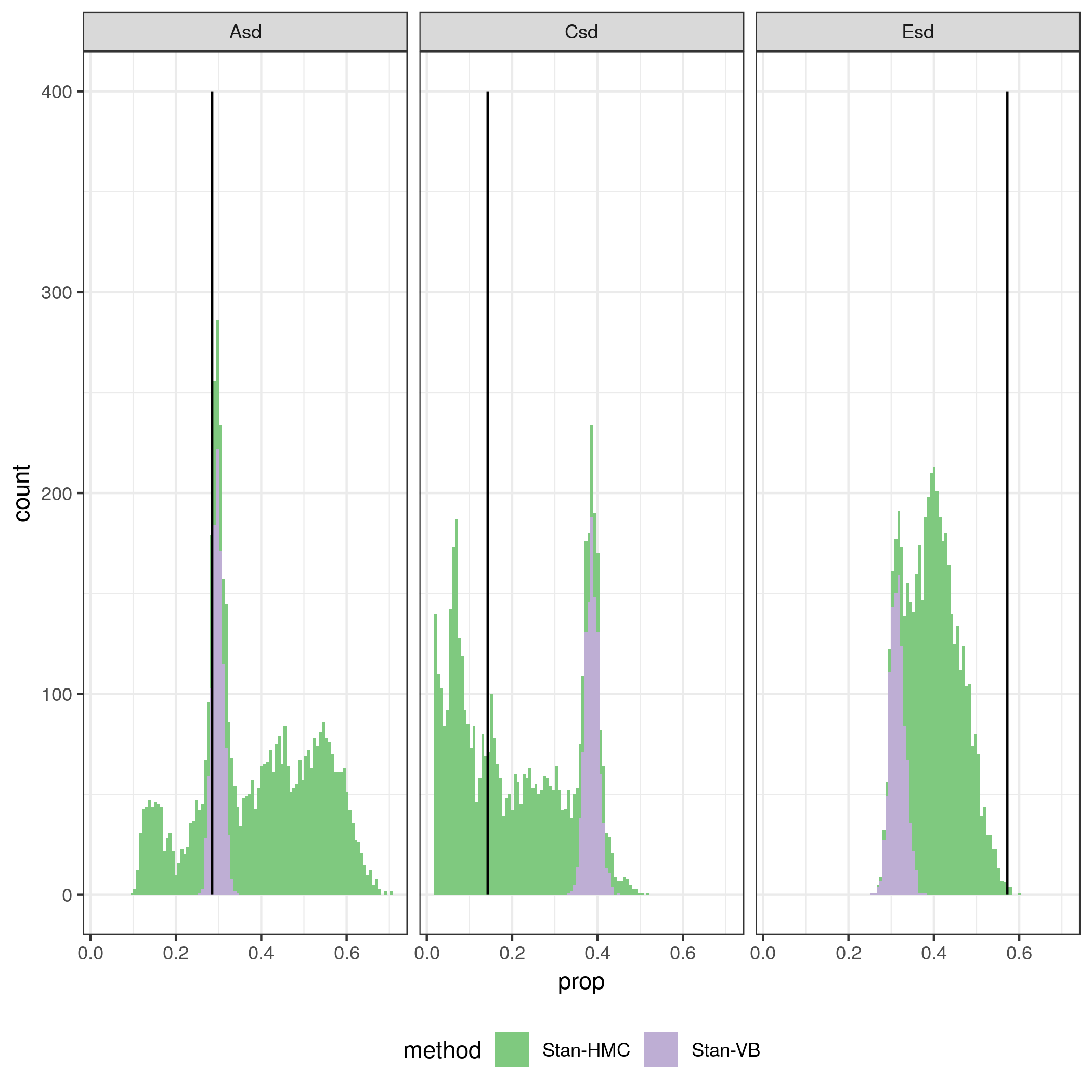
Quickly I ran into problems with speed with the Stan’s Hamiltonian MC method. So I tried the variational bayes method (which I don’t really know anything about) as well. It is much faster! Variational bayes is about ten times faster than the MCMC procedure. But it is also quite a bit off! The figure below show 1000 draws from the posterior distributions of variance components A, C and E obtained with regular Stan Hamiltonian MC and variational bayes. The trade-off between speed and quality is there for everyone to see. The A component seems reasonably well estimated in VB (but it is known for underestimating the variance), but for the C component it is quite off.

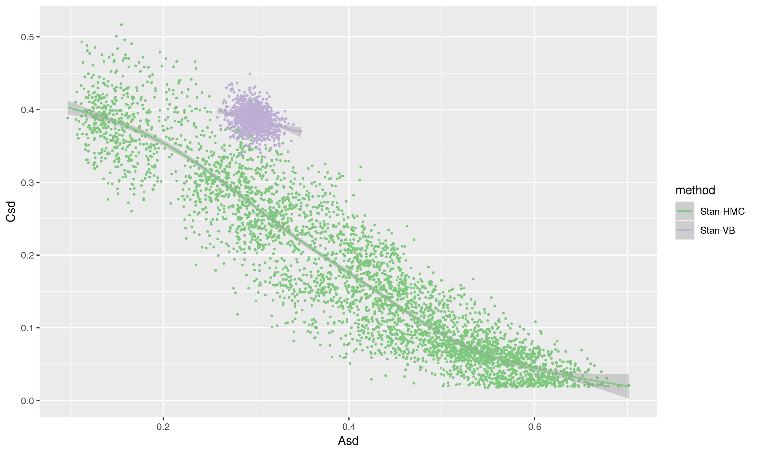
The scatterplot below shows the same draws, with A and C plotted on the x and y axes respectively. The VB method clearly yields results very different from the HMC, and the likely underestimation of the variance in the posterior means it is a no, no for future use (except perhaps for debugging).

---